PMCTrack-GUI is a Python front-end for the pmctrack command-line tool. This application extends the capabilities of the PMCTrack stack with features such as an SSH-based remote monitoring mode or the ability to plot the values of user-defined performance metrics in real time. This GUI application runs on Linux and Mac OS X. More information on how to install PMCTrack and PMCTrack-GUI can be found here.
Getting started with PMCTrack-GUI
To start using PMCTrack-GUI run the pmctrack-gui launcher located in ${PMCTRACK_ROOT}/src/gui/.
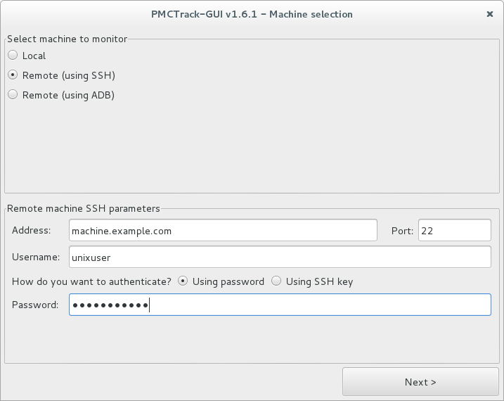
As shown in the figure above, the initial window makes it possible to choose the machine to be monitored. This machine can be:
-
The actual system running PMCTrack-GUI (local machine).
-
Any other machine accessible via SSH. In this option, certain connection parameters located in the bottom half of the window must be provided. These parameters include the hostname or IP address of the target machine, the port number associated with the SSH server, the user name and password (or the SSH key alternatively).
-
Any other machine accessible via ADB-server. In order to monitor a remote machine using an ADB-server, you must first prepare the ADB-server so you can access the machine to be monitored by “adb shell” from the server. In addition, it is necessary that external requests can be made through the port destined to it (default 5037), for it is sufficient that run the following command at the ADB-server:
$ socat TCP-LISTEN:5037,reuseaddr,fork UNIX-CLIENT:/tmp/5037Once this is done, you just have to specify the hostname or IP address of the ADB-server and the port number (default 5037) in PMCTrack-GUI window.
To continue click on the “Next” button on the lower right corner of the window. If the connection to the target machine was successful (if an error is encountered, the user will be properly notified), PMCTrack-GUI detects the features and capabilities of the target machine (architecture, processor model, number of hardware counters available, total number of CPUs, etc). Once the information has been retrieved, a new window will be displayed.
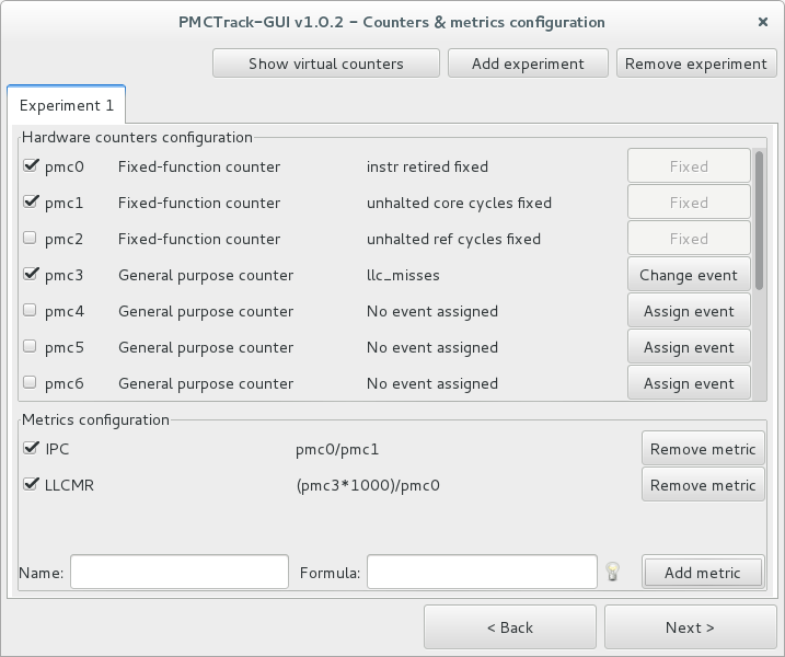
This new window, shown above, enables the user to configure hardware performance counters, virtual counters as well as the high-level metrics whose values will be later plotted in graphs updated in real time.
Monitored hardware events are organized in separate sets. Henceforth, we will refer to these sets as experiments. When using various experiments, different event sets are monitored in a round-robin fashion (event multiplexing); this enables to use the same physical counter to monitor different hardware events belonging to different experiments. The two buttons on the top right corner of the window make it possible to add or delete experiments. At least one experiment must be configured. In case many experiments are created, information on each experiment will be displayed in a separate tab.
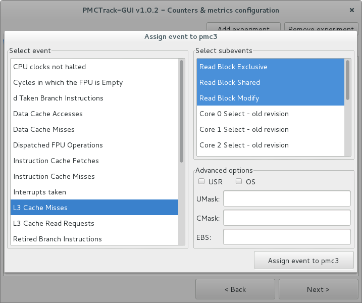
Two types of hardware counters exist: fixed counters, –always associated with a specific event–, and general-purpose counters, which can be assigned different events to be monitored. Activating a fixed hardware counter boils down to checking their corresponding checkbox. (Note that some processor models, such as most AMD multicore processors, do not feature fixed-function counters). To activate a general-purpose hardware counter, a hardware event must be assigned to it first. To do so, click on the “Assign event” button; a dialog window will appear, enabling to select events and sub-events from a list. Multiple sub-events of a specific event can be selected by holding the Ctrl key, as shown in the following figure.
Once the user has selected the desired hardware events, it is now time to define a set of high-level metrics. A different set of high-level metrics exists for each experiment. As such, high-level metrics must be defined in terms of performance counters used in the same experiment. To illustrate the simplicity behind the definition of high-level metrics, let us consider the following example. Suppose that we are using the first HW counter (pmc0) to monitor retired instructions, and the second one (pmc1) to count elapsed clock cycles. In this case, we can easily define the Instructions per Cycle (IPC) metric with the following formula: pmc0/pmc1. More complex formulas can be used, such as ((pmc0+pmc1)^pmc4)/(pmc6*pmc7).
On some modern systems, PMCTrack allows to count events that are not exposed to the OS via hardware monitoring counters. This is the case of temperature readings or power/energy consumption measurements. These kind of “unconventional” hardware events are exposed by PMCTrack as virtual counters. Overall, virtual counters are always assigned the same event and do not belong to any specific experiment. If virtual counters are available on the target machine (an PMCTrack implements it), a button called “Show virtual counters” will be displayed on the window. When clicking on the button, a list of available virtual counters and associated events will be displayed. Note that these counters can be also used to define high-level metrics associated with any experiment. To make this possible, the right ‘virtX’ variable must be used to refer to a specific virtual counter. For example, the following formula defines a high-level metrics in terms of the first virtual counter virt0: (pmc0+pmc1)/virt0. Notably, in defining a high-level metric, only those virtual counters and hardware counters with the associated checkbox activated can be used.
Once hardware/virtual counters and metrics have been properly set up, we may click on the “Next” button. In doing so, a new window will appear, such as the one shown below:
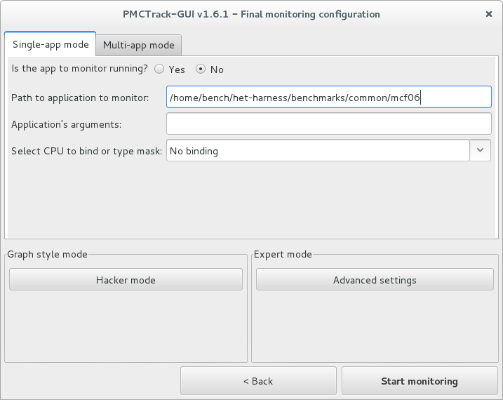
This window allows to set up the remaining parameters of the monitoring session. Settings are divided into the following three sections:
-
Single-app/Multi-app mode: Used to specify the application(s) to monitor. In single-app mode, you can monitor an application to run at that time, specifying the path to the application, its arguments (if any) and, optionally, the CPU(s) to bind the application to; or an application that is already running, specifying the PID of the application and, optionally, the CPU(s) to bind the application to. In multi-app mode, you can launch a number of applications sequentially, so you can view monitoring data in real time of the running application (like in single-app mode) and the final monitoring data of the applications whose execution has been completed (like in single-app mode when the application is finished). Paths to applications to monitor along with their arguments must be specified in a file (one line per application).
-
Graph style mode selection: Used to customize the visual aspect of performance graphs. Predefined styles (default mode, aqua mode, hacker mode, etc) or custom styles can be selected. You may change the style of a particular graph later during the monitoring session by clicking on the graph.
-
Advanced settings: Used to perform specific adjustments on the monitoring session.
- Pmctrack command: Specify the path to pmctrack command (established to ‘pmctrack’ by default).
- Samples configuration: Specify the sampling period for hardware counters and virtual counters (1000ms by default), as well as the size of the kernel buffer used to store samples (unspecified by default).
- Counter mode selection: Specify the choice for the monitoring mode. Two modes are supported: per-thread mode (mode by default) or system-wide mode (on a per-CPU basis).
- Save monitoring logs into files: These options make it possible to save gathered monitoring data in text files (logs). Currently two logging modes are supported: (1) save the value of performance/virtual counters or (2) save the values of the user-defined high-level metrics (both logging modes disabled by default).
Once these settings have been properly specified, the user may click on the “Start monitoring” button found at the bottom right corner of the window. In doing so, the specified application will be launched on the target machine (unless application is already running) and a monitoring window, such as the one shown below, will appear. (If you chose the Multi-app mode, a window with the list of applications appears, by clicking on each of these applications you will access the corresponding monitoring window)
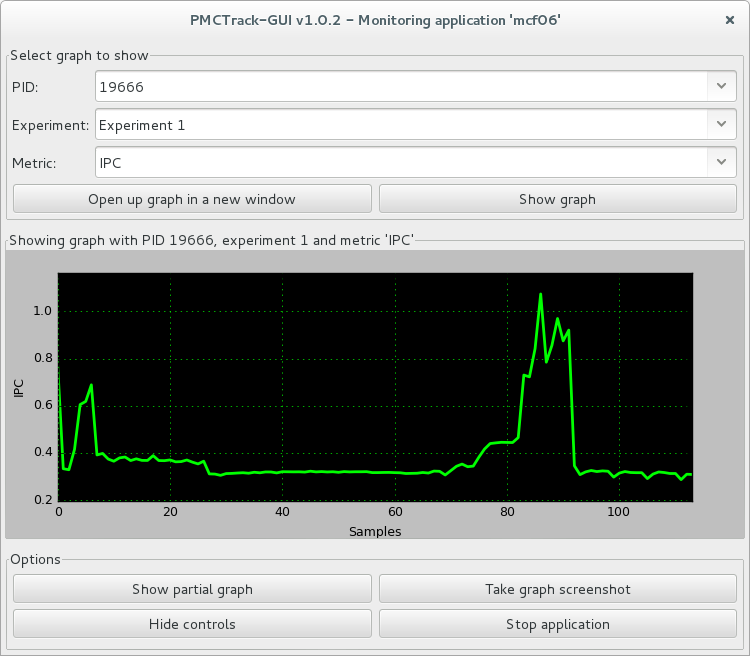
A monitoring windows allow viewing a performance graph updated in real time. As evident, the window is divided into three parts. The upper part features controls for specifying what is actually being displayed in the graph (thread’s PID in per-thread mode or CPU in system-wide mode, experiment number and specific high-level metric). When setting up this information, the user may opt to either update the graph on the current monitoring window or create a new monitoring window to display the information. This allows to visualize multiple performance graphs updated simultaneously in real time. The central part of a monitoring window displays a performance graph. The windows’s title indicates the information being displayed (PID/CPU, the experiment number and the name of the metric). Finally, the bottom of a monitoring window includes various controls that allow the user to perform different actions:
- Show complete graph: view the current part of the monitoring or cumulative graph.
- Take graph screenshot: save the current graph as an image.
- Hide controls: hide the controls so that the graph ocuppies the entire window space.
- Stop application: pause the monitoring session. It can be then resumed at any time.
Notably, in the middle of a monitoring session, the user can set up another monitoring session by browsing the various configuration windows shown earlier.